

Table of Contents
ToggleI remember the first time I was handed a spreadsheet with thousands of rows of information. It was a complete and utter mess. Columns were half-empty, some numbers were formatted as text, and the sheer volume of it all made my head spin. I felt like I was standing in front of a giant, cluttered storeroom, and I had been tasked with organizing it all by hand. The thought of finding a single, specific piece of information, let alone uncovering a hidden trend within that chaos, felt impossible.
That feeling—the overwhelming sense of being lost in a sea of data—is something I know many people experience. It’s what stopped me from diving into data analysis for a long time. I believed you had to be a mathematical genius or a coding wizard to make sense of it. But then I discovered something that changed everything for me. It wasn’t a secret formula or a magic spell. It was a tool, a simple-sounding thing called Pandas.
Pandas isn’t some complex, intimidating program. Basically, it’s a friendly assistant, a digital spreadsheet on steroids that lives inside your computer. It takes that giant, messy storeroom of data and gives you the tools to clean it, organize it, and find the stories hidden within it. It’s the closest thing to a superpower I’ve ever found for working with data.
If you’re just starting out, if you feel the same way I did—overwhelmed and a little intimidated—then this guide is for you. I’m going to walk you through my own personal journey with Pandas, from the very first steps to the moment I felt like I could truly master my data.
Understanding the Big Idea: What Is Pandas, Really?
Before we even touch a line of code, let’s understand what Pandas is. Imagine you have a notebook. One type of page in this notebook is a single column of information—a list of names, a list of ages, a series of temperatures. In Pandas, this is called a Series. It’s the simplest building block, like a single column in your spreadsheet.
Now, imagine a full-page spreadsheet with multiple columns and rows, complete with headers. This is the main player in Pandas, the DataFrame. It’s the workhorse that lets you store, organize, and manipulate your data. Think of it as that entire cluttered storeroom I mentioned, but now you have a powerful set of tools to sort through every shelf and box.
Pandas gives you a simple way to create these DataFrames and Series, and then provides hundreds of easy-to-use methods for working with them.
My First Steps: Setting Up My Workspace
Getting started with Pandas is surprisingly simple. You just need to have Python installed on your computer. If you’ve got that, you’re halfway there. The first thing I did was open my terminal or command prompt and type a single command to get the Pandas library:
pip install pandas
After that, every time I wanted to use Pandas in a new project, I just had to do one more thing at the very top of my code. It’s a simple, familiar ritual now.
import pandas as pd
That little “as pd” part is a convention in the data world. It’s like giving your assistant a nickname. Instead of typing pandas every time, you just type pd. It saves a ton of time and makes your code a lot cleaner.
My First Data: Building a Personal DataFrame
To learn how to use Pandas, I had to create some data of my own. I didn’t want to just copy something from a textbook; I wanted to work with something real and personal. So, I decided to create a list of my favorite movies and their ratings. It was a simple project, but it taught me everything.
I created a dictionary in Python, which is a collection of key-value pairs. Think of it like a list of column headers and the data that goes with each one.
import pandas as pd
my_movies = {
'Title': ['Inception', 'The Matrix', 'Parasite', 'Spirited Away', 'Pulp Fiction'],
'Director': ['Christopher Nolan', 'The Wachowskis', 'Bong Joon Ho', 'Hayao Miyazaki', 'Quentin Tarantino'],
'Year': [2010, 1999, 2019, 2001, 1994],
'My_Rating': [9.5, 9.0, 9.8, 10.0, 9.3]
}
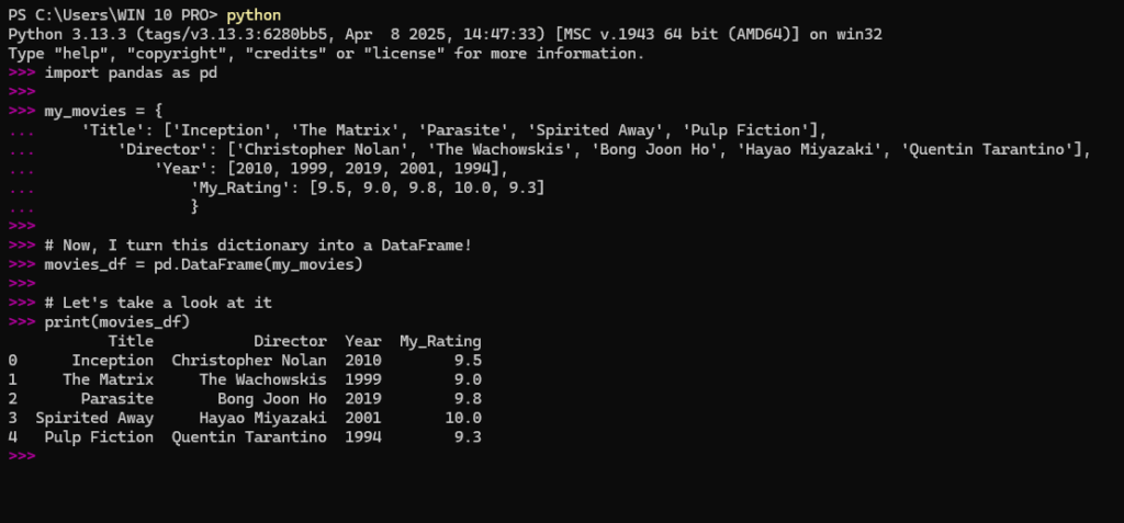
# Now, I turn this dictionary into a DataFrame!
movies_df = pd.DataFrame(my_movies)
# Let's take a look at it
print(movies_df)
When I ran that code, a beautiful, organized table appeared in my console. It was perfect. I had just created my first DataFrame, and it felt like a small triumph.
Here is the screenshot of output when I run this code:
I quickly learned two essential commands for viewing my data. If I had a huge dataset and just wanted a sneak peek, head() and tail() were my best friends.
					# Show the first 3 rows
print(movies_df.head(3))

# Show the last 2 rows
print(movies_df.tail(2))
Here is the screenshot of the output:
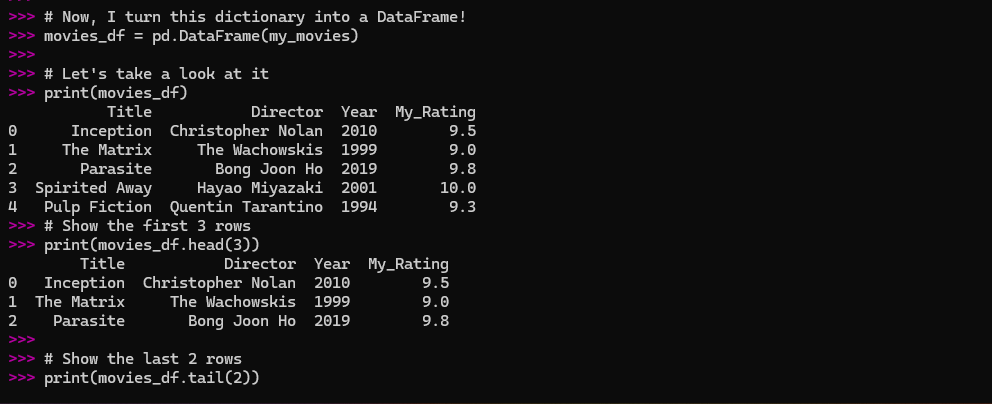
This was a much more manageable way to deal with a lot of information than just printing the whole thing.
The Art of Selection: Finding a Needle in a Haystack
Now that I had my data, I needed to learn how to get specific pieces of it. This is where Pandas truly shines. It’s like having a master key to every drawer in my digital storeroom.
Finding a Single Column
The easiest way to pull out a single column (a Series) is to use the column name inside square brackets.
					# Get just the movie titles
movie_titles = movies_df['Title']
print(movie_titles)
Here is the screenshot of the output:
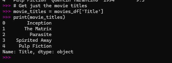
This gave me a clean list of just the titles. It’s so much simpler than going through the entire spreadsheet and manually copying them.
Finding Multiple Columns
What if I wanted just the ‘Title’ and ‘My_Rating’? All I had to do was pass a list of the columns I wanted.
					# Get just the movie titles
movie_titles = movies_df['Title']
print(movie_titles)
Here is the screenshot of output:
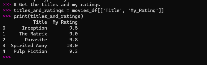
The double brackets are a common point of confusion for beginners. Just remember: one set of brackets to get a single Series, and two sets to get a new DataFrame with multiple columns.
Selecting Rows: Location is Everything
This is where I first got a little confused, but once I understood the logic, it became second nature. Pandas has two main ways to select rows:
loc(short for ‘location’): This is for when you want to find data by its label or name. For a DataFrame, the labels are the row numbers, starting from 0.iloc(short for ‘integer location’): This is for when you want to find data by its position or integer index.
Let’s use my movies DataFrame as an example.
# I want the movie at the second position (which is at index 1)
# I use iloc because I care about the position
print(movies_df.iloc[1])
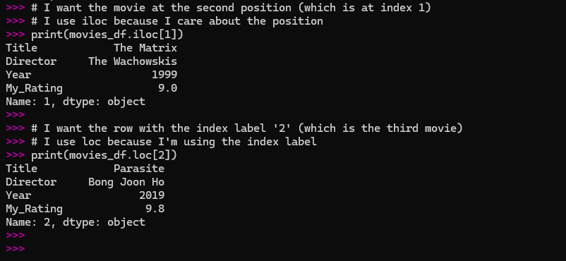
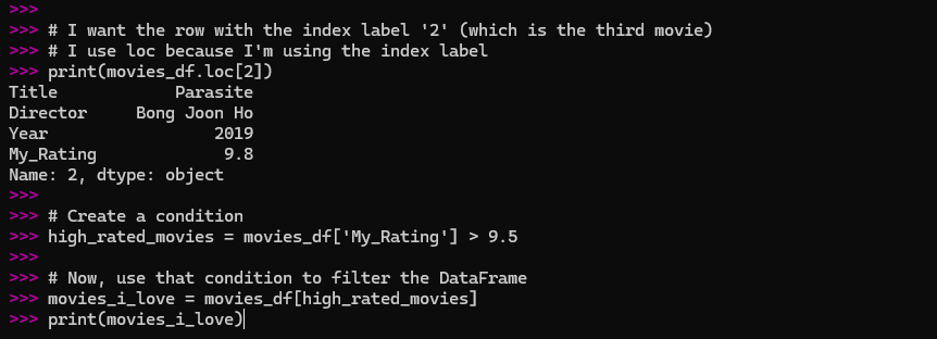
# I want the row with the index label '2' (which is the third movie)
# I use loc because I'm using the index label
print(movies_df.loc[2])
Here is the screenshot of the output:
I found it helpful to think of it like this: loc is like asking a person by name, and iloc is like asking the person in the third seat from the front.
The Power of Filtering
This is probably the most useful thing I learned early on. Instead of manually looking through my list of movies, I could tell Pandas to show me only the ones that met a certain condition.
Let’s say I wanted to see only the movies I rated above 9.5.
					# Create a condition
high_rated_movies = movies_df['My_Rating'] > 9.5

# Now, use that condition to filter the DataFrame
movies_i_love = movies_df[high_rated_movies]
print(movies_i_love)
Here is the screenshot of the output:
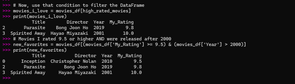
This single line of code gave me a new DataFrame with just ‘Spirited Away’ and ‘Parasite’. It felt incredibly powerful.
You can combine conditions with & (and) and | (or).
					# Movies I rated 9.5 or higher AND were released after 2000
new_favorites = movies_df[(movies_df['My_Rating'] >= 9.5) & (movies_df['Year'] > 2000)]
print(new_favorites)
Here is the screenshot of the output:
This showed me just ‘Parasite’ and ‘Spirited Away’, because ‘Inception’ was released in 2010 but its rating was exactly 9.5, not higher.
Cleaning Up the Mess: A Real-World Problem
Not all data is as neat as my movie list. In fact, most of it is messy. Missing data is a constant challenge. I decided to simulate this by creating a new DataFrame about my friends’ favorite foods, but with a few blank spots.
					my_friends_foods = {
    'Name': ['Sarah', 'David', 'Chris', 'Maria', 'Alex'],
    'Favorite_Food': ['Pizza', 'Tacos', None, 'Sushi', 'Pasta'],
    'Meal_of_Day': ['Lunch', 'Dinner', 'Breakfast', 'Dinner', 'Lunch']
}

friends_df = pd.DataFrame(my_friends_foods)

print(friends_df)
Here is the screenshot of the output:
					my_friends_foods = {
    'Name': ['Sarah', 'David', 'Chris', 'Maria', 'Alex'],
    'Favorite_Food': ['Pizza', 'Tacos', None, 'Sushi', 'Pasta'],
    'Meal_of_Day': ['Lunch', 'Dinner', 'Breakfast', 'Dinner', 'Lunch']
}

friends_df = pd.DataFrame(my_friends_foods)

print(friends_df)
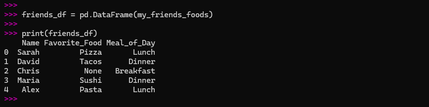
As you can see, Chris’s favorite food is missing. Pandas represents this with NaN (Not a Number), which basically means “nothing here.”
Finding Missing Data
Pandas has a simple way to find these missing values: isnull().
print(friends_df.isnull())
Here is the screenshot of the output:
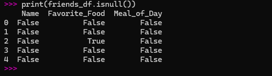
This returns a DataFrame of True and False values, where True means a value is missing. It’s a great way to quickly see where the gaps are.
Filling in the Gaps
I had two choices for dealing with Chris’s missing data:
Remove the row entirely: The
dropna()method is perfect for this. It removes any row that has a missing value.
					# Remove any row with a missing value
cleaned_df = friends_df.dropna()
print(cleaned_df)
Here is the screenshot of the output:
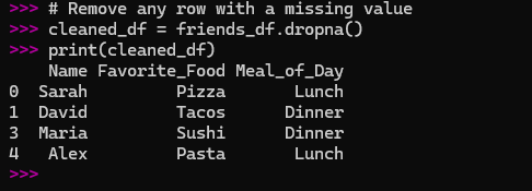
This is useful if you have a huge dataset and a small number of missing values.
Fill the missing value: The
fillna()method lets you replaceNaNwith something else.
					# Fill in the missing value with a placeholder
filled_df = friends_df.fillna('Not Specified')
print(filled_df)
Here is the screenshot of the output:
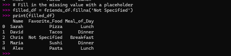
This is great for keeping all your data, even if it’s incomplete.
This simple exercise taught me that I didn’t have to manually go through and fix every problem. Pandas could do it for me in a single line of code.
Adding New Information: Creating New Columns
My next step was to realize that I could create new columns from the data I already had. It’s like adding a new section to my spreadsheet and having Pandas automatically fill it out based on a rule I provide.
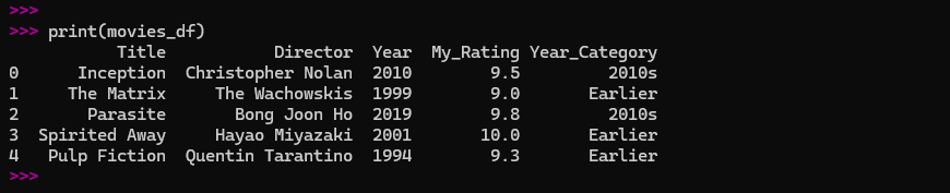
Using my movie DataFrame, I decided to create a new column called ‘Year_Category’ to label movies as ‘2010s’ or ‘1990s’.
					# Create a new column with a simple rule
movies_df['Year_Category'] = movies_df['Year'].apply(lambda x: '2010s' if x >= 2010 else 'Earlier')

print(movies_df)
I had just added a whole new dimension to my data, and I didn’t have to manually type anything. This felt like a huge leap in my understanding.
Doing the Math: Finding Hidden Insights
Now for the fun part: using Pandas to do quick calculations and find surprising insights.
Let’s go back to my movie data.
					# What's my average rating?
average_rating = movies_df['My_Rating'].mean()
print(f"My average rating for these movies is: {average_rating}")

# What's the highest rating I gave?
highest_rating = movies_df['My_Rating'].max()
print(f"The highest rating I gave is: {highest_rating}")
These simple functions (mean(), max(), min(), sum()) are the cornerstone of any data analysis.
But the most useful function I discovered for quick summaries was describe(). It gives you a whole bunch of statistical information all at once.
print(movies_df.describe())
This printed out a table with the count, average, standard deviation, and a bunch of other useful numbers for every numerical column. It was a one-stop shop for a quick overview of my data.
Grouping for Insights: The Power of groupby()
The groupby() method is one of the most powerful tools in Pandas, and it’s also one of the most intimidating for a beginner. But once you get the hang of it, it’s like a whole new world opens up.
The concept is simple: you want to group your data by a certain characteristic and then perform a calculation on each group. The data science community has a saying for this: “split-apply-combine.”
Split: You split the data into groups based on a column.
Apply: You apply a function (like finding the average or the count) to each group.
Combine: You combine the results into a new DataFrame.
Let’s use a new, slightly different dataset. I’ll imagine I’m tracking my daily steps and hours of sleep for a week.
					activity_data = {
    'Day': ['Mon', 'Tue', 'Wed', 'Thu', 'Fri', 'Sat', 'Sun'],
    'Activity_Type': ['Work', 'Work', 'Rest', 'Work', 'Work', 'Rest', 'Rest'],
    'Steps': [7500, 8100, 2500, 9200, 7800, 12000, 5000],
    'Sleep_Hours': [7.5, 7.8, 8.5, 7.2, 7.6, 9.0, 8.1]
}

activity_df = pd.DataFrame(activity_data)
print(activity_df)

# I want to know my average steps and sleep hours on 'Work' days vs. 'Rest' days.
average_by_activity = activity_df.groupby('Activity_Type').mean()
print(average_by_activity)
The result was a beautiful, clean table showing me the average steps and sleep hours for each type of day. The groupby() function did all the heavy lifting, splitting the data, calculating the averages for each group, and putting it all back together.
My First Real Project: A Step-by-Step Walkthrough
To put everything I’d learned into practice, I decided to do a simple end-to-end project. I would create a small dataset about my plants, clean it, analyze it, and draw some conclusions.
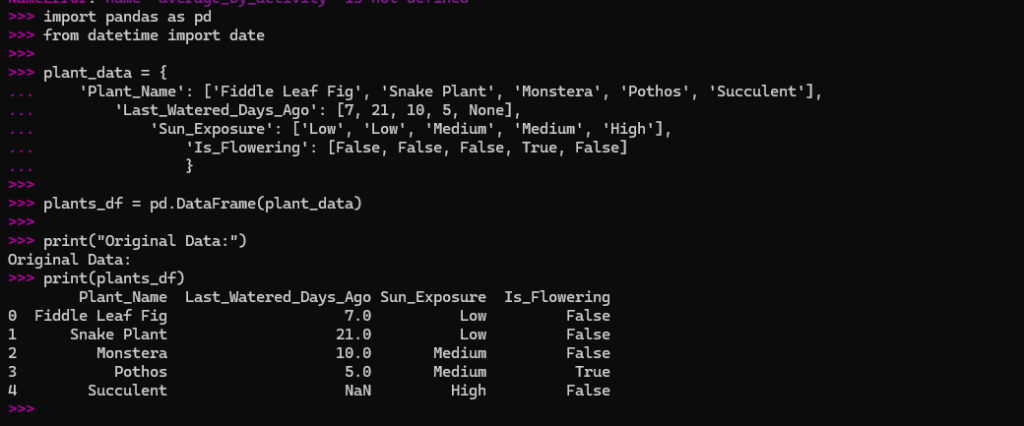
Step 1: Creating the Raw Data
I decided to track the last time I watered my plants, the type of plant, and how much sun they get.
					import pandas as pd
from datetime import date

plant_data = {
    'Plant_Name': ['Fiddle Leaf Fig', 'Snake Plant', 'Monstera', 'Pothos', 'Succulent'],
    'Last_Watered_Days_Ago': [7, 21, 10, 5, None],
    'Sun_Exposure': ['Low', 'Low', 'Medium', 'Medium', 'High'],
    'Is_Flowering': [False, False, False, True, False]
}

plants_df = pd.DataFrame(plant_data)

print("Original Data:")
print(plants_df)
Here is the screenshot of the output:
Step 2: Finding and Handling Missing Data
I immediately saw that I didn’t remember when I last watered the succulent. I knew this was a good opportunity to use fillna(). Since it’s a succulent and doesn’t need much water, I’ll just fill it with a high number.
					plants_df['Last_Watered_Days_Ago'] = plants_df['Last_Watered_Days_Ago'].fillna(30)

print("\nData after filling missing value:")
print(plants_df)
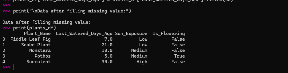
Now my data is complete and clean.
Step 3: Doing Some Simple Math
I wanted to know the average number of days since I last watered my plants.
					average_watering = plants_df['Last_Watered_Days_Ago'].mean()

print(f"\nOn average, my plants were last watered {average_watering:.2f} days ago.")
The screenshot of above calculation:
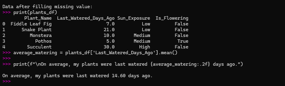
The .2f just made the number a bit cleaner, rounding it to two decimal places.
Step 4: Grouping for Deeper Insights
I had a feeling that plants with different sun exposures might have different watering needs. I used groupby() to test this.
					avg_watering_by_sun = plants_df.groupby('Sun_Exposure')['Last_Watered_Days_Ago'].mean()

print("\nAverage watering days by sun exposure:")
print(avg_watering_by_sun)
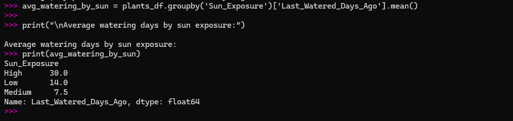
The results showed that plants with ‘Low’ sun exposure were watered less frequently than those with ‘Medium’ or ‘High’ exposure. This confirmed my suspicion and gave me a concrete piece of information from my data.
Step 5: Filtering for a Specific Condition
Finally, I wanted to see which plants needed watering soon. I decided to filter for any plant that was watered more than 6 days ago.
					needs_watering = plants_df[plants_df['Last_Watered_Days_Ago'] > 6]

print("\nPlants that need watering soon:")
print(needs_watering)
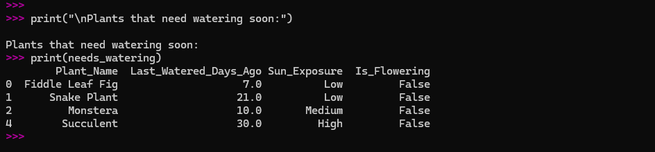
The result showed me my Fiddle Leaf Fig and Monstera. It was a simple, practical use of filtering that helped me solve a real-world problem.
My Final Thoughts and Encouragement
Looking back at that overwhelming spreadsheet I started with, I can see how far I’ve come. Pandas didn’t just teach me how to write code; it taught me a new way of thinking. It showed me that data isn’t a chaotic mess to be feared, but a collection of stories waiting to be told.
The secret to mastering it isn’t to memorize every command. It’s to understand the core concepts and to start small. Don’t worry about being perfect. Just create some simple data, mess around with it, and ask it questions. Try to find an answer to a question you have about your own life, your hobbies, or your work.
Pandas is a tool that empowers you to turn confusion into clarity. It can take a cluttered desk and make it a neat, organized workspace where you can find everything you need. It’s a journey, and every line of code you write is a small step forward. So, go ahead. Open a new notebook, import Pandas, and start your own adventure. You might be surprised by the stories you find.
Explore further into the fascinating world of python by reading my main pillar post: Python For AI – My 5 Years Experience To Coding Intelligence

Stay ahead of the curve with the latest insights, tips, and trends in AI, technology, and innovation.